Description of the problem
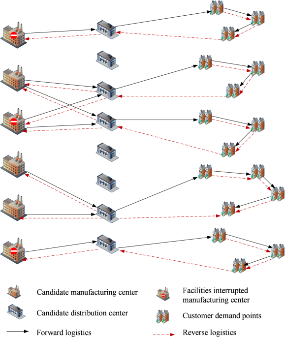
The traditional supply chain is dominated by a linear, single-directional hierarchical structure, emphasizing the logistics sequential flow among suppliers, manufacturers, and distributors, and the model mostly focuses on the cost-efficiency optimization of production, storage, and transportation. The e-commerce closed-loop supply chain, on the contrary, relies on the Internet platform and is characterized by order-driven, bi-directional logistics (forward delivery and reverse return) and multi-level node collaboration, and needs to simultaneously deal with the risks of dynamic demand, uncertain return rates and facility disruptions. In the model construction, the e-commerce supply chain focuses more on uncertainty modeling and the overall optimization of the supply chain network, and the mathematical complexity is significantly higher than that of the traditional model. The e-commerce closed-loop supply chain structure is shown in Fig. 1, the e-commerce closed-loop supply chain network is simplified to include manufacturing centers, distribution centers, and customer demand points. In the forward logistics flow, products are transported from manufacturing centers to various distribution centers, and then distribution centers provide delivery services to customer points. In reverse logistics, the returned and exchanged products from customer points are first collected at the distribution center for inspection and processing, and then the parts of products that need to be returned to the manufacturing center are transported to the manufacturing center for repair and reprocessing, form a secondary closed-loop supply chain network for recycling from the point of demand to the distribution center to the manufacturing center. The uncertainty factors include customer demand and reverse returns, while also considering the risk of facility disruption at the manufacturing center. In the background of carbon policy, the government has formulated relevant carbon quota policies, and enterprises reduce carbon emissions through green upgrading and transformation. Decision makers need to make decisions on facility location and facility relationship allocation, product flow allocation, transportation routes, and emission reduction technology investment plans for uncertain closed-loop supply chain networks.
Closed-loop supply chain network structure diagram.
Problem assumptions
-
a.
Customer demand for a single variety of products.
-
b.
The locations of the potential manufacturing centers, distribution centers, and customers are known.
-
c.
Each customer point is served by only one distribution center, and the returned and exchanged products of each customer point are still recovered by the distribution route they serve.
-
d.
Each manufacturing center selects only one level of investment in emission reduction technologies.
-
e.
Some of the returned products at the customer’s point have quality defects, which are inspected by the distribution center and returned to the manufacturing center for repair. The return rate of returned products is known, and the repaired products re-enter the sales network with no difference in quality from the new products.
Description of symbols
(a) Description of the collection.
I: Candidate manufacturing center collection,\(i \in I\)
J: Candidate distribution center collection,\(j \in J\)
K: Demand point collection,\(k \in K\)
S: Manufacturing center facility outage scenario collection,\(s \in S\)
L: Collection of different types of delivery vehicles,\(l \in L\)
R: Investment grade collection of emission reduction technology,\(r \in R\)
(b) Definition of parameters.
Fi: Manufacturing Center i construction costs.
Fj: Construction costs of distribution center j.
MFi: Manufacturing Center i Production costs per unit of product.
VFj: Distribution center j Recycling and processing costs per unit of product.
RMFi: Manufacturing Center i Repair unit product production costs.
TCl: Transport vehicle type l Unit transport costs.
TCij: Unit product transportation costs from manufacturing center i to distribution center j.
TCjk: Unit transportation cost from distribution center j to demand point k.
ai: The state parameters of manufacturing center i; the normal operation of the manufacturing center is 1; otherwise, it is 0.
pi: Manufacturing center i Probability of facility disruption.
bi: Manufacturing Center i Proportion of capacity remaining after an disruption has occurred.
FC: Fixed costs for the construction of facilities.
MC: Production costs for manufacturing centers and repair costs for returned products.
VC: Distribution center recycling and disposal costs.
GC: Technology input costs for abatement in manufacturing centers.
TC: Transport costs.
CFi: Manufacturing center i fixed CO2 emissions from construction.
MQi: Manufacturing center i CO2 emissions per unit of product produced.
r: Investment grade for abatement technologies.φ: Investment grade cost factors for abatement technologies.
air: Proportion of carbon emissions reduced per unit of product produced in manufacturing center i with an emissions reduction investment grade r.
CFj: Distribution center j fixed CO2 emissions from construction.
RQj: Distribution center j CO2 emissions from recycled goods disposal units of product.
FCE: Fixed carbon emissions from facility construction.
MCE: Carbon emissions from production processes.
VCE: Total carbon emissions from the recycling inspection process.
TCE: Carbon emissions from transport.
\(\mu _j\): Distribution center j Return rate of returned products.
\(C_i^\hboxmax \): Manufacturing center i capacity limit.
\(C_l^\hboxmax \): Vehicles l Loading capacity limit.
\(C_j^\hboxmax \): Capacity limit for distribution center j.
\(C_jv^\hboxmax \): Maximum recycling capacity of distribution center j.
disij: Distance from manufacturing center i to distribution center j.
TQl: Transport vehicle type l Carbon dioxide emissions per kilometer of product transported.
\(\widetilde d_k\): Customer demand points k Actual market demand.
\(\widetilde e_k\): Customer demand point k Actual number of returned products.
Elim: Carbon emission allowances.
(c) Decision-making variables.
\(X_i = \left\{ \beginarrayll\text1, & \textSelect manufacturing center i \\ \text, & \textOtherwise \endarray \right. , i \in \operatornameI\)
\(Y_j=\left\{ \beginarray*20c \text1,&\textSelect distribution center j \\ \text0,&\textOtherwise \endarray \right. , j \in J\)
\(\begingathered Z_l=\left\{ \beginarray*20c \text1&\textIf the vehicle l\text is used for transportation \\ \text&\textOtherwise \endarray \right.,l \in L \hfill \\ \hfill \\ \endgathered\)
\(X_ir=\left\{ \beginarray*20c \text1&\begingathered \textInvestment in emission reduction technology \hfill \\ \textwith grade r\text for manufacturing center i \hfill \\ \endgathered \\ \text&\textOtherwise \endarray \right.,i \in I\)
\(X_ij^s=\left\{ \beginarray*20c \text1&\begingathered \textThe manufacturing center i\text and the \hfill \\ \textdistribution center j\text establish a supply \hfill \\ \textrelationship under the scenario s \hfill \\ \endgathered \\ \text&\textOtherwise \endarray \right.,i \in I,j \in J,s \in S\)
\(Y_jk=\left\{ \beginarray*20c \text1,&\textCustomer k\text is served by the distribution center j \\ \text0,& \textOtherwise \endarray \right. , j \in J,k \in K\)
\(Y_kk’^j=\left\{ \beginarray*20c 1&\begingathered \textThere is a path between customer k\text and \hfill \\ \textcustomer k’ \text,when k=0\text,it represents \hfill \\ \textthe distribution center j\text. \hfill \\ \endgathered \\ 0&\textOtherwise \endarray \right.,j \in J,k \in K,k’ \in K\)
\(V_ij^s\): The number of products supplied by manufacturing center i to distribution center j under scenario s.
\(V_ijl^s\): The number of products provided by vehicle l from manufacturing center i to distribution center j under scenario s.
\(V_jil^s\): The number of maintenance products of vehicle l from distribution center j to manufacturing center i under scenario s.
Vjkl: The number of products transported by vehicle l from distribution center j to demand point k.
Vkjl: The number of returned goods of vehicle l from demand point k to distribution center j.
Ykk’jl: vehicle l from distribution center j first service customer k to customer k’..
Model construction
Economic objective function construction
The first objective function Z1 aims to minimize the total cost of the network, which is expressed as follows:
(a) Fixed construction cost of facilities:
$$FC=\sum\limits_i Fi \cdot Xi+\sum\limits_j Fj \cdot Yj $$
(1)
In this equation, the first term represents the fixed construction cost of manufacturing centers, and the second term represents the fixed construction cost of distribution centers.
(b) Production costs at manufacturing centers and repair costs for returned/exchanged products:
$$MC=\sum\limits_i,j,s,l (V_ijl^s – V_jil^s) \cdot MFi+V_jil^s \cdot RMF$$
(2)
(c) Recycling and processing costs at distribution centers:
$$VC=\sum\limits_k,j,l Vkjl \cdot VFj$$
(3)
(d) Emission reduction technology investment costs at manufacturing centers:
$$GC=\sum\limits_i,r Xir \frac12\varphi r^2$$
(4)
To accelerate the achievement of low-carbon goals, green upgrades, and transformations will be implemented in existing technologies at manufacturing centers. r indicates the level of r emission reduction technology investment for manufacturing center i, and \(1/2\varphi r^2\) is an increasing convex function concerning the level of emission reduction technology investment; that is, the higher the level of emission reduction technology input at node facilities is, the greater the cost of emission reduction technology input and the lower the carbon emissions produced during product production.
(e) Transport costs:
$$\begingathered TC=\sum\limits_i,j,s,l \left\lceil V_ijl^s/C_l^\hboxmax \right\rceil \cdot disij \cdot TCl+\sum\limits_j,k,l \left\lceil Vjkl/C_l^\hboxmax \right\rceil \cdot Ykk’jl \cdot disjk \cdot TC l \hfill \\ \text +\sum\limits_j,k,k^\prime ,l \left\lceil Vkjl/C_l^\hboxmax \right\rceil \cdot Ykk’jl \cdot disjk \cdot TCl+\sum\limits_i,j,s,l \left\lceil V_jil^s/C_l^\hboxmax \right\rceil \cdot disij \cdot TCl \hfill \\ \endgathered$$
(5)
In the equation, the first term represents the forward logistics transportation cost from manufacturing center i to distribution center j; the second term represents the forward logistics transportation cost from distribution center j to demand point k; the third term represents the reverse logistics transportation cost for return and exchange products from demand point k to distribution center j; and the fourth term represents the reverse logistics transportation cost for products requiring return to the manufacturing center i for repair, from distribution center j to manufacturing center i.
In summary:
$$Z1=\hboxmin (FC+MC+VC+GC+TC)$$
(6)
Economic objective function construction
The second objective function of Z2 is to minimize carbon emissions, which is expressed as follows:
(a) Fixed carbon emissions from facility construction:
$$FCE=\sum\limits_i CFi \cdot X_i +\sum\limits_j CFj \cdot Yj$$
(7)
In the equation, the first term represents the fixed carbon emissions from the construction of the manufacturing center, and the second term represents the fixed carbon emissions from the construction of the distribution center.
(b) Carbon emissions generated during the production process:
$$MCE=\sum\limits_i,j,s,l V_ijl^s \cdot [(1 – Xir)+Xir \cdot (1 – air)] \cdot MQ_i$$
(8)
(c) Total carbon emissions generated during the recycling and inspection process:
$$VCE=\sum\limits_k,j,l V_kjl \cdot RQ_j$$
(9)
(d) Carbon emissions generated during transportation:
$$\begingathered TCE=\sum\limits_i,j,s,l \left\lceil V_ijl^s/C_l^\hboxmax \right\rceil \cdot TQl \cdot disij+\sum\limits_j,k,l \left\lceil Vjkl/C_l^\hboxmax \right\rceil \cdot TQl \cdot Ykk’jl \cdot disjk \hfill \\ \text +\sum\limits_j,k,l \left\lceil Vkjl/C_l^\hboxmax \right\rceil \cdot TQl \cdot Ykk’jl \cdot disjk+\sum\limits_i,j,s,l \left\lceil V_jil^s/C_l^\hboxmax \right\rceil \cdot TQl \cdot disij \hfill \\ \endgathered$$
(10)
In the equation, the first term represents the carbon emissions generated during the transportation of products from distribution center i to distribution center j; the second term represents the carbon emissions generated during transportation from distribution center j to demand point k; the third term represents the carbon emissions generated during the transportation of returned products from demand point k to distribution center j; the fourth term represents the carbon emissions generated during the transportation of returned products requiring factory repairs from distribution center j to manufacturing center i.
In summary:
$$Z2=\hboxmin (FCE+MCE+VCE+TCE)$$
(11)
Constraint condition
To ensure the feasibility and practicality of the model, several constraint conditions must be satisfied:
(a) Logical relationship constraints:
Equations (12)–(14) represent the logical constraints of the model. Equation (12) indicates that only open manufacturing centers can provide services to distribution centers. Equation (13) specifies that only open distribution centers can serve customer points. Equation (14) is the emission reduction technology investment constraint, stating that each manufacturing center can only invest in one level of emission reduction technology.
$$X_ij^s \leqslant X_i,\forall i \in I,j \in J,s \in S$$
(12)
$$Y_jk \leqslant Y_j,\forall j \in J$$
(13)
$$\sum\limits_r X_ir \leqslant 1,\forall i \in I$$
(14)
(b) Network logistics balance constraints:
Equations (15)–(18) are the network logistics balance constraints. Equation (15) ensures that all products produced at manufacturing centers are transported to the distribution centers. Equation (16) ensures that the total transportation volume of products at distribution centers meets the forward logistics demand of all customer points. Equation (17) ensures that the total amount of returned products meets the reverse logistics demand of customer points. Equation (18) ensures that products that qualify for remanufacturing are sent to manufacturing centers for remanufacturing.
$$\sum\limits_i,l V_ijl^s =\sum\limits_k,l V_jkl ,\forall j \in J,s \in S$$
(15)
$$\sum\limits_j,l V_jkl \geqslant \sum\limits_k \widetilde d_k \cdot Y_jk,\forall j \in J,k \in K$$
(16)
$$\sum\limits_j,l V_kjl \geqslant \sum\limits_k \in K \widetilde e_k \cdot Y_jk,\forall j \in J,k \in K$$
(17)
$$\sum\limits_i,l V_jil^s =\sum\limits_j,l V_kjl \cdot \mu ,\forall j \in J,\forall k \in K,\forall l \in L$$
(18)
(c) Facility capacity constraints:
Equations (19)–(21) are the facility capacity constraints. Equation (19) ensures that the production quantity at the manufacturing center does not exceed its production capacity. Equation (20) ensures that the volume of products flowing into the distribution center does not exceed its maximum capacity. Equation (21) ensures that the volume of recovered products at the distribution center does not exceed its maximum recovery capacity.
$$\sum\limits_j,l V_ijl^s \leqslant [\alpha _si \cdot C_i^\hboxmax +(1 – \alpha _si) \cdot C_i^\hboxmax \cdot b_i] \cdot X_i,\forall i \in I,j \in J,l \in L$$
(19)
$$\sum\limits_k,l V_jkl \leqslant C_j^\hboxmax \cdot Y_j,\forall j \in J,k \in K,l \in L$$
(20)
$$\sum\limits_k,l V_kjl \leqslant C_jv^\hboxmax \cdot Y_jk,\forall j \in J,k \in K,l \in L$$
(21)
(d) Vehicle routing planning constraints:
Equation (22) to (24) are vehicle routing constraints. Equations (22) and (23) specify that each delivery only serves one demand point, meaning each customer is only served once. Equation (24) ensures that each distribution center serves only the customers assigned to it.
$$\sum\limits_k Y_kk’^j =1,\forall Y_kj=1,Y_k’j=1,k \ne k’$$
(22)
$$\sum\limits_k’ Y_kk’^j =1,\forall Y_kj=1,Y_k’j=1,k \ne k’$$
(23)
$$\sum\limits_k,k’ Y_kk’jl \leqslant Y_jkl,\forall j \in J,l \in L$$
(24)
(e) Carbon emission limit constraints:
Equation (25) ensures that the total carbon emissions of the closed-loop supply chain do not exceed the government-mandated limit.
$$FCE+MCE+VCE+TCE \leqslant E_\lim $$
(25)
(f) Decision variable constraints:
Equations (26) and (27) are the decision variable constraints.
$$X_i,X_ij^s,Y_j,Y_jk,Y_kk’jl,Z_l \in \ 0,1\ ,\forall i \in I,j \in J,k \in K,k’ \in K,l \in L$$
(26)
$$V_ijl^s,V_jil^s,V_jkl,V_kjl \geqslant 0,\forall i \in I,j \in J,k \in K,s \in S,l \in L$$
(27)
Uncertain requirements handling
For uncertain customer point demand \(\widetilde d_k\) and uncertain return quantity \(\widetilde e_k\), box uncertainty sets are used to describe uncertain parameters. The variables \(\Gamma _k^d\) and \(\Gamma _k^e\)are introduced to control the level of uncertainty in both forward and reverse logistics demand. \(\Gamma _k^d\) represents the number of variations in forward logistics demand at customer points, while \(\Gamma _k^e\)represents the number of variations in reverse logistics demand, the range of values is within the interval of [0, |K|]. Based on the robust optimization approach proposed by Bertsimas D and Sim M39, the robust counterpart of the constraint Eqs. (16) and (17) containing uncertain parameters was obtained:
$$\sum\limits_k d_k \cdot Y_jk+p_k\Gamma _k^d+\sum\limits_k z_k \leqslant \sum\limits_j,l V_jkl ,\forall j \in J,k \in K$$
(28)
subject to
$$p_k+z_k \geqslant \widehat d_k \cdot Y_jk,\forall k \in K$$
(29)
$$p_k \geqslant 0,z_k \geqslant 0,\forall k \in K$$
(30)
$$\sum\limits_k e_k \cdot Y_jk+r_k\Gamma _k^e+\sum\limits_k t_k \leqslant \sum\limits_j,l V_kjl ,\forall j \in J,k \in K,l \in L$$
(31)
subject to
$$r_k+t_k \geqslant \widehat e_k \cdot Y_jk,\forall k \in K$$
(32)
$$r_k \geqslant 0,t_k \geqslant 0,\forall k \in K$$
(33)
Facility state description method
For the description of the facility state, Wang Zhijin et al.40 reflect the uncertainty of the system by constructing different scenario sets to provide a reasonable depiction of the possible future situations or consequences caused, which is suitable for dealing with uncertainties with unknown probability distribution functions or discrete uncertainties, and describes the multiple future state values of the uncertain system by using the qualitative analysis method to analyze the future state values in a quantitative way. In this study, the scenario method is used to describe the facility disruption scenarios at manufacturing centers, with the production status of the manufacturing center represented by the parameter ai.
$$\alpha _i=\left\{ \beginarray*20c \text1,&\textThe manufacturing center i operation normally \\ \text0,&\textThe manufacturing center i operation interruption \endarray \right.$$
(34)
Assuming that the probabilities of a facility outage at each manufacturing center are independent of each other and that the likelihood of an outage at i for a manufacturing center is pi, the probability that the manufacturing center will function normally is 1-pi. Assuming a total of S outage scenarios, the probability ps of the occurrence of the scenario\(s(s \in S)\) is as follows:
$$p_s=\prod\limits_m \in I p_i \prod\limits_i \in I (1 – p_i)$$
(35)
In the formula, m is the manufacturing center where the disruption occurred.
In summary, the robust model of an uncertain closed-loop supply chain network in a carbon policy context proposed in this paper is as follows:
$$\hboxmin ( Z_1,Z_2)$$
(36)